Clustering Networks for Enterprise Application Management

5 min read

Peeling back the layers of any company’s IT operations reveals a network of applications and services that form the functional basis of any modern enterprise: directory services, accounting applications, CRMs—the picture becoming more or less complex with the industry and level of technology adoption. Through our project work at CKM Analytix, we’ve discovered that the key to answering questions about a company’s technology ecosystem relies on its mathematical framing. For example, one client of ours is in the process of planning a multi-year effort to deconstruct and transfer the majority of its internally-managed applications to new sites. The significant operational risk of this endeavor can be mitigated with data science, namely, by leveraging the concept of an enterprise technology ecosystem as a graph of applications. Applications (or app tiers, virtualized servers, platforms, etc.) are represented by the nodes of this graph, while operational data that describes their interdependency forms their edges. This graph data structure enables a group of data scientists to powerfully analyze the systems and visualize the world-map of the client’s application space.

In our actual use case, an intermediary step is to group systems into local clusters that rely on each other. Perhaps technical debt and poor design led to overuse of multi-tenancy, or the requirements of some services include a high volume and low-latency channel with an upstream data source. Both situations imply these applications form a community which ought to have their interdependency respected in the event of a major change. The layout of this problem has several well-documented analogues. Take, for instance, a program that can be decomposed into a set of processes and points of communication between them. In order to efficiently parallelize this program, our scheme should minimize communication between CPUs while distributing the computational load as evenly as possible across the available cores. Thus, we represent the program as a graph of nodes (the discrete processes) and edges (the points at which these processes must exchange information). By clustering the program’s tasks into groups of high intercommunication, we’ve found a reasonable scheme for distributing a program over many compute resources. If we substitute the program in this case for an entire space of applications, the same approach generally applies.

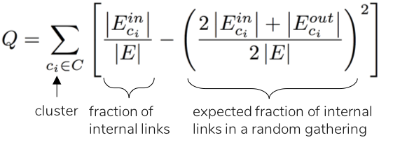
Based on the field of applications and the problem under study, the associated dataset can be clustered using models like K-Means, Spectral Clustering, Girvan-Newman technique, etc., which are often implemented using a graph data structure. To reiterate, we connect two nodes by an edge if the nodes have some relation. A clustering technique forms clusters by applying labels to nodes such that edges are broken (preferably weaker ones) if the breaking optimizes the metric of interest (objective function). One of the metrics that gained popularity in the recent past is modularity [6], which relies on the notion that when nodes are linked in a random way, they do not form clusters. Therefore, modularity-based clustering detects a group of nodes as a cluster when the nodes inside the group have more internal links (edges) compared to that of a random gathering with the same degree sequence. The mathematical expression of modularity is given as [6]:

To illustrate modularity-based clustering, consider the American College Football Network shown below [4]. Each node in this network represents a football team, and an edge between two teams indicates that these teams played a game against each other. The ground truth indicates that the teams are divided into twelve clusters, which represent the various football leagues and are shown below by different colors.

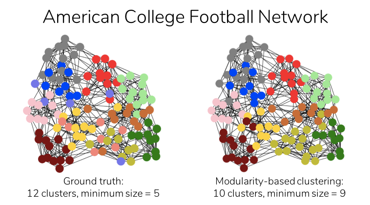
On using modularity-based clustering to the above football network, only ten communities (minimum cluster size: 9 football teams) are generated, as opposed to twelve in the ground truth (minimum size: 5 teams). This is a result of the resolution limit problem, which modularity-based clustering often suffers from [3]. This refers to the tendency to merge clusters of size smaller than a certain threshold with larger ones. To resolve this resolution limit problem, modularity is rescaled using scale ‘r’ as [1]

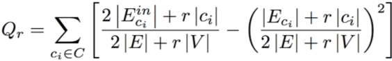
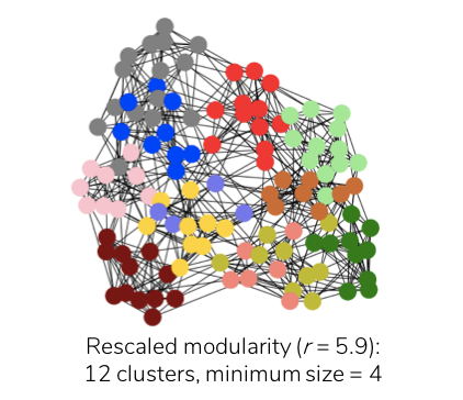
where a larger resolution ‘r’ results in better detection of smaller clusters. Therefore, applying rescaled modularity-based clustering (at ‘r’ = 5.9) to the football network now generates twelve clusters, which is consistent with the ground truth, with the smallest cluster comprising four nodes as illustrated below.

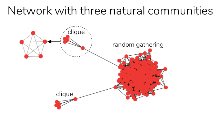
In addition to the resolution limit problem, the metric modularity suffers from another opposing problem, particularly in heterogenous networks (i.e. networks comprising communities of varied sizes) [5]. For example, consider the following heterogenous network, consisting of three natural communities: two cliques and a random gathering, which are loosely linked to one another.

On applying modularity-based clustering to the above network, the resultant clusters are shown below at both higher and lower resolutions of rescaled modularity, depicting the two opposing problems of modularity.

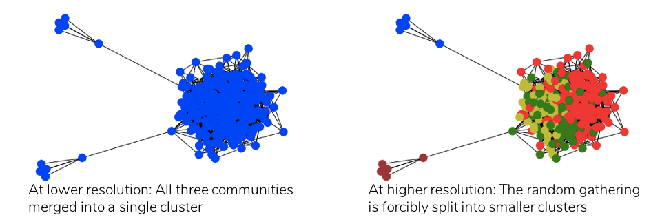
While the two small cliques merge into the large cluster at lower resolution (resolution limit problem), at higher resolution, the larger cluster is forcibly split into smaller ones. In fact, no value of the resolution scale ‘r’ exists such that the above three natural communities are identified as three separate clusters.

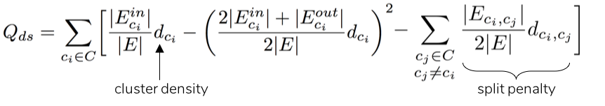
In order to resolve these two coexisting problems of modularity (i.e., the problem of favoring larger clusters at lower resolution and smaller clusters at higher resolution), another metric called modularity density is introduced by Chen et al. (2014) [2]. Modularity density introduces additional components, such as split penalty and cluster density, to the mathematical expression of modularity [2]:

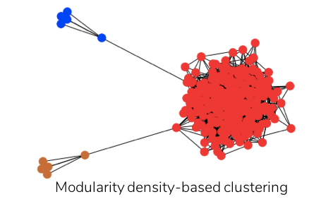
While split penalty helps resolve the tendency to split larger clusters, cluster density disfavors the formation of smaller clusters. On applying modularity density-based clustering to the above heterogenous network, the three natural communities are successfully identified as three separate clusters as illustrated below.

Therefore, clustering using modularity density-based partitioning instead of modularity provides a more meaningful community structure to the network, especially when there is a wide distribution of cluster sizes. However, modularity density performs at the expense of higher computational cost compared to that of modularity.

Consider the composition of the graph in the example problem posed at the beginning of this article. A set of servers supporting the functions of an application may form a small community, as in the simplest case of a set of webservers behind a load balancer, while a platform may form a web of relations that encompasses an entire operational unit. From the networking perspective, compute resources are often segmented into secure compartments bridged by DMZs. If we took these networked compartments as ground truth clusters, any significant variation in the size of these compartments would make the modularity metric-based clustering insufficient for capturing the quality of our clusters. Thus, our experience leads us to the conclusion that the enterprise application space tends towards heterogeneity, particularly as the scope of the data widens and the ground truth represents a complex, sprawling technology unit. Given this heterogeneity, we recommend modularity density-based maximization and related techniques for mining groups from infrastructure datasets.

For Python implementations of the clustering techniques described above, CKM has published an open source repository containing fine-tuned optimization algorithms as described by Chen et al. [2]. These algorithms form clusters by optimizing modularity or modularity density. As an extension to the original work by Chen et al., CKM also provides clustering algorithms that not only optimize the desired metric, but also account for any user-specified thresholds on maximum community size. Such an extension better fits these algorithms for enterprise applications. For further details, refer to the CKM Analytix open source project.

REFERENCES

[1] ARENAS A, FERNANDEZ A, GOMEZ S. Analysis of the structure of complex networks at different resolution levels. New Journal of Physics, vol. 10, no. 5, p. 053039, 2008.

[2] CHEN M, KUZMIN K, SZYMANSKI BK. Community detection via maximization of modularity and its variants. IEEE Transactions on Computational Social Systems. 1(1), 46–65, 2014.

[3] FORTUNATO S, BARTHELEMY M. Resolution limit in community detection. Proceedings of the National Academy of Sciences, vol. 104, no. 1, pp. 36–41, 2007.

[4] GIRVAN M, NEWMAN MEJ. Community structure in social and biological networks. Proceedings of the National Academy of Sciences, vol. 99, no. 12, pp. 7821–7826, 2002.

[5] LANCICHINETTI A, FORTUNATO S. Limits of modularity maximization in community detection. Physical Review E, vol. 84, no. 6, p. 066122, 2011.

[6] NEWMAN MEJ, GIRVAN M. Finding and evaluating community structure in community structure in networks. Physical Review E, vol. 69, p. 026113, 2004.